Github Repo | Full-code notebook

In this post, I will work my way into basic Sentiment Analysis methods and experiment with some techniques. I will use the data from the IMDB review dataset acquired from Kaggle.

We will be examining/going over the following:

  • Data preprocessing for sentiment analysis
  • 2 different feature representations:
    • Sparse vector representation
    • Word frequency counts
  • Comparison using:
    • Logistic regression
    • Naive Bayes

Feature Representation

Your model will be, at most, as good as your data, and your data will be only as good as you understand them to be, hence the features. I want to see the most useless or naive approaches and agile methods and benchmark them for both measures of prediction success and for training and prediction time.

Before anything else, let’s load, organize and clean our data really quick:

 1
 2
 3
 4
 5
 6
 7
 8
 9
10
11
12
13
14
15
16
17
18
19
20
21
22
23
24
import CSV

def get_data():
    with open('data/kaggle_data/movie.csv', 'r') as f:
        data = list(CSV.reader(f, delimiter=','))
    return data

def split_data(data):
    # split 80/10/10
    train_split = int(0.8 * len(data))
    val_split = int(0.9 * len(data))
    return data[:train_split], data[train_split:val_split], data[val_split:]

def save_data(data, filename):
    with open(filename, 'w') as f:
        writer = csv.writer(f)
        writer.writerows(data)

def main():
    data = get_data()
    train, val, test = split_data(data[1:])
    save_data(train, 'data/train.csv')
    save_data(val, 'data/val.csv')
    save_data(test, 'data/test.csv')

Let’s start with creating a proper and clean vocabulary that we will use for all the representations we will examine.

Clean Vocabulary

We just read all the words as a set, to begin with,

1
2
3
4
5
6
7
# Get all the words
words = [w for s in train_data for w in s[0].split()]
# len(words) = 7391216

# Get the vocabulary
dirty_vocab = set(words)
# len(dirty_vocab) = 331056

So for the beginning of the representation, we have 331.056 words in our vocabulary. This number is every non-sense included, though. We also didn’t consider any lowercase - uppercase conversion. So let’s clean these step by step.

1
2
3
4
5
6
7
8
9
# Convert to lowercase
vocab = set([w.lower() for w in dirty_vocab])
# len(vocab) = 295827

# Remove punctuation
from nltk.tokenize import RegexpTokenizer
tokenizer = RegexpTokenizer(r'\w+')
vocab = set([w.lower() for w in tokenizer.tokenize(' '.join(vocab))])
# len(vocab) = 84757

We reduced the number from 331.056 to 84.757. We can do more. With this method, we encode every word we see in every form possible. So, for example, “called,” “calling,” “calls,” and “call” will all be a separate words. Let’s get rid of that and make them reduce to their roots. Here we start getting help from the dedicated NLP library NLTK since I don’t want to define all these rules myself (nor could I):

1
2
3
4
5
# Reduce words to their stems
from nltk.stem import PorterStemmer
stemmer = PorterStemmer()
vocab = set([stemmer.stem(w) for w in vocab])
# len(vocab) = 58893

The last step towards cleaning will be to get rid of stopwords. These are ’end,’ ‘are,’ ‘is,’ etc. words in the English language.

1
2
3
4
5
6
7
8
# Remove connectives
import nltk
nltk.download('stopwords')

from nltk.corpus import stopwords
stop_words = set(stopwords.words('English))
vocab = vocab - stop_words
# len(vocab) = 58764

Now that we have good words, we can set up a lookup table to keep encodings for each word.

1
2
# Vocabulary dictionary
vocab_dict = {w: i for i, w in enumerate(vocab)}

Now we have a dictionary for every proper word we have in the data set. Therefore, we are ready to prepare different feature representations.

Since we will convert sentences in this clean form, again and again, later on, let’s create a function that combines all these methods:

 1
 2
 3
 4
 5
 6
 7
 8
 9
10
11
12
13
14
15
16
17
# Function to combine all the above to clean a sentence
def clean_sentence(sentence):
    # Convert to lowercase
    sentence = sentence.lower()
    # Words
    words = sentence.split()
    # Remove punctuation
    tokenizer = RegexpTokenizer(r'\w+')
    words = tokenizer.tokenize(' '.join(words))
    # Remove stop words
    stop_words = set(stopwords.words('English))
    words = [w for w in words if w not in stop_words]
    # Reduce words to their stems
    stemmer = PorterStemmer()
    words = [stemmer.stem(w) for w in words]
    # remove repeated words
    return set(words)

Ideally, we could initialize tokenizer stemmer and stop_words globally (or as a class parameter), so we don’t have to keep initializing.

Sparse Vector Representation

This will represent every word we see in the database as a feature… Sounds unfeasible? Yeah, it should be. I see multiple problems here. The main one we all think about is this is a massive vector for each sentence with a lot of zeros (hence the name). This means most of the data we have is telling us practically the same thing as the minor part; we have these words in this sentence vs. we don’t have all these words. Second, we are not keeping any correlation between words (since we are just examining word by word).

We go ahead and create a function for encoding every word for a sentence:

1
2
3
4
5
6
7
8
9
# function to convert a sentence to a vector encoding
def encode_sparse(sentence):
    words = sentence.split()
    vec = np.zeros(len(vocab))
    clean_words = clean_sentence(sentence)
    for w in clean_words:
        if w in vocab_dict:
            vec[vocab_dict[w]] += 1
    return vec

We then convert all the data we have using this encoding (in a single matrix):

1
2
train_data_sparse = np.array([encode_sparse(s[0]) for s in train_data]), np.array([int(s[1]) for s in train_data])
val_data_sparse = np.array([encode_sparse(s[0]) for s in val_data]), np.array([int(s[1]) for s in val_data])

That’s it for this representation.

Word Frequency Representation

This version practically reduces the 10.667 dimensions to 3 instead. We are going to count the number of negative sentences a word passes in as well as positive sentences. This will give us a table indicating how many positive and negative sentences a word has found in:

1
2
3
4
5
6
7
# Counting frequency of words
freqs = np.zeros((len(vocab), 2)) # [positive, negative]
for i, s in enumerate(train_data):
    words = clean_sentence(s[0])
    for w in words:
        if w in vocab_dict:
            freqs[vocab_dict[w], int(s[1])] += 1

The next thing to do is to convert these enormous numbers into probabilities. There are multiple points to add here: First, we are getting the probability of this single word being in many positive and negative sentences, so the values will be minimal. Hence we need to use a log scale to avoid floating point problems. Second is, we might get words that don’t appear in our dictionary, which will have a likelihood of 0. Since we don’t want a 0 division, we add laplacian smoothing, like normalizing all the values with a small initial. Here goes the code:

1
2
# Convert to log probabilities with Laplace smoothing
freqs = np.log((counts + 1) / (np.sum(counts, axis=0) + len(vocab)))

After getting the frequencies and fixing the problems we mentioned, we now define the new encoding method for this version of the features

1
2
3
4
5
6
7
8
def encode_freq(sentence):
    words = clean_sentence(sentence)
    vec = np.array([1., 0., 0.]) # [bias, positive, negative]
    for word in words:
        if word in vocab_dict:
            vec[1] += freqs[vocab_dict[word], 0]
            vec[2] += freqs[vocab_dict[word], 1]
    return vec

We end by converting our data as before

1
2
train_data_pos_neg = np.array([encode_freq(s[0]) for s in train_data]), np.array([int(s[1]) for s in train_data])
val_data_pos_neg = np.array([encode_freq(s[0]) for s in val_data]), np.array([int(s[1]) for s in val_data])

Let’s take a sneak peek at what our data looks like:

 1
 2
 3
 4
 5
 6
 7
 8
 9
10
11
12
13
14
15
16
17
18
19
20
21
22
23
24
25
# Visualize the data with PCA
from sklearn.decomposition import PCA
import matplotlib.pyplot as plt
%matplotlib inline

# Create a PCA instance. 
# This will reduce the data to 2 dimensions 
# as opposed to 3, where we have 2 features and a bias, more on that in next episode.
PCA = PCA(n_components=2)

# Fit the PCA instance to the training data
x_data = train_data_pos_neg[0]
PCA.fit(x_data)

# Transform the training data to 2 dimensions ignoring the bias. This is due to the fact that the bias is a constant and will not affect the PCA
x_data_2d = PCA.transform(x_data)
plt.scatter(x_data_2d[:, 0], x_data_2d[:, 1], c=train_data_pos_neg[1], cmap='bwr')
plt.xlabel('First Principal Component')
plt.ylabel('Second Principal Component')

# Setup legend
import matplotlib.patches as mpatches
red_patch = mpatches.Patch(color='red', label='Negative')
blue_patch = mpatches.Patch(color='blue', label='Positive')
plt.legend(handles=[red_patch, blue_patch])

Untitled

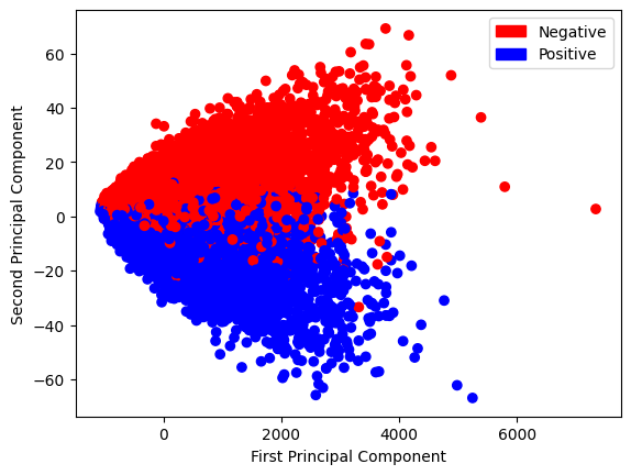
A better would be to use PCA for this kind of representation, but for now, we will ignore that fact since we want to explore that in episode 2.

Model Development

This episode mainly focuses on cleaning the data and developing decent representations. This is why I will only include Logistic Regression for representation comparison, we then can compare Naive Bayes and Logistic Regression to pick a baseline for ourselves.

Logistic Regression

Logistic regression is a simple single-layer network with sigmoid activation. This is an excellent baseline as it is one of the simplest binary classification methods. I am not explaining this method in depth, so if you want to learn more, please do so. I will use a simple PyTorch implementation.

1
2
3
4
5
6
7
class LogisticRegression(nn.Module):
    def __init__(self, input_dim):
        super(LogisticRegression, self).__init__()
        self.linear = nn.Linear(input_dim, 1)
        
    def forward(self, x):
        return torch.sigmoid(self.linear(x))

We then define the loss function and the optimizer to use. I am using Binary Cross Entropy for the loss function and Adam for the optimization with a learning rate of 0.01.

 1
 2
 3
 4
 5
 6
 7
 8
 9
10
11
12
13
14
15
16
17
18
19
20
21
22
23
24
25
26
27
28
29
30
device = torch.device('cuda' if torch.Cuda.is_available() else 'CPU')
model = LogisticRegression(x_data.shape[1]).to(device)
optimizer = optim.Adam(model.parameters(), lr=0.01)
criterion = nn.BCELoss()

# Train the model
num_epochs = 100
train_loss = []
val_loss = []
for epoch in range(num_epochs):
    # Forward pass
    outputs = model(X_train)
    loss = criterion(outputs, y_train.unsqueeze(1))
    
    # Backward and optimize
    optimizer.zero_grad()
    loss.backward()
    optimizer.step()
    
    train_loss.append(loss.item())
    
    # Validation
    with torch.no_grad():
        outputs = model(X_val)
        loss = criterion(outputs, y_val.unsqueeze(1))
        val_loss.append(loss.item())
    
    if (epoch) % 100 == 0:
        print ('Epoch [{}/{}], Loss: {:.4f}' 
               .format(epoch, num_epochs, loss.item()))

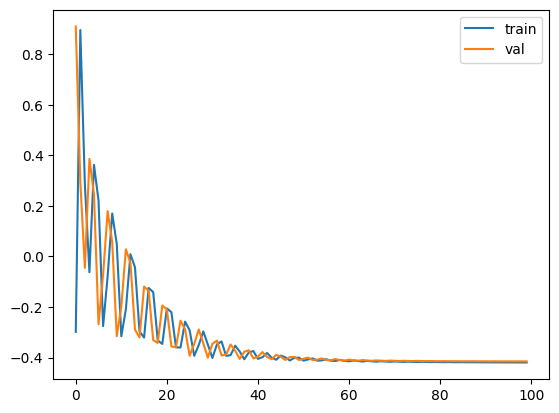
Sparse Representation Training We first start with training the sparse representation. I trained for 100 epochs and reached 0.614 training accuracy and 0.606 validation accuracy. Here is the learning curve

Untitled

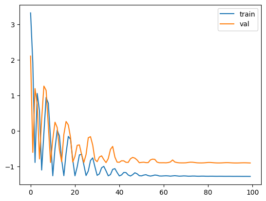
Word Frequency Representation Training I trained using the same parameter settings above, reaching 0.901 training accuracy and 0.861 validation accuracy. Here is the learning curve in the log scale

Untitled

Naive Bayes

The next really good baseline is Naive Bayes. This is a very simple model that is very fast to train and has a very good accuracy. Naive Bayes is a probabilistic model that uses Bayes’ theorem to calculate the probability of a class given the input. The main assumption of this model is that the features are independent of each other. This is why it is called Naive. To give a basic intuition of how this model works, let’s say we have a sentence I love this movie and we want to classify it as positive or negative. We first calculate the probability of the sentence being positive and negative using the conditional frequency probability we calculated above and multiply them by the prior probability of the class. The class with the highest probability is the predicted class.

To put it in other terms, this is the Bayes Rule:

$$P(C|X) = \frac{P(X|C)P(C)}{P(X)}$$

We then calculate $P(w_i|pos)$ and $P(w_i|neg)$ for each word in the sentence where $w_i$ is the $i^{th}$ word in the sentence and $pos$ and $neg$ are the positive and negative classes respectively. We then multiply the ratio of these, so:

$$\prod_{i=1}^{n} \frac{P(w_i|pos)}{P(w_i|neg)}$$

If the result is greater than 1, we predict the sentence to be positive, otherwise negative. When we convert this to log space and add the log prior, we get the Naive Bayes equation:

$$\log \frac{P(pos)}{P(neg)} + \sum_{i=1}^{n} \log \frac{P(w_i|pos)}{P(w_i|neg)}$$

We now implement this in python and numpy.

 1
 2
 3
 4
 5
 6
 7
 8
 9
10
11
12
13
14
15
16
17
18
19
20
21
22
23
24
25
26
27
28
29
30
31
32
33
34
35
36
37
38
39
40
41
42
43
44
45
# Naive Bayes model (vanilla implementation)
class NaiveBayes:

    def __init__(self, num_classes=2):
        self.num_classes = num_classes

    def fit(self, X, y):
        # Log Prior: num_pos/num_neg
        num_pos = (y == 1).sum()
        num_neg = (y == 0).sum()
        self.log_prior = np.log(num_pos/num_neg)

        # Frequency table for words
        self.lambda_ = {}
        for i, data in enumerate(X):
            sentence = clean_sentence(data)
            label = int(y[i])
            for j, word in enumerate(sentence):
                if word not in self.lambda_:
                    self.lambda_[word] = np.zeros(self.num_classes)
                self.lambda_[word][label] += 1
        
        # Convert to word probabilities with Laplace smoothing
        N_pos = sum([self.lambda_[word][1] for word in self.lambda_])
        N_neg = sum([self.lambda_[word][0] for word in self.lambda_])
        V = len(self.lambda_)
        for word in self.lambda_:
            self.lambda_[word][1] = (self.lambda_[word][1] + 1) / (N_pos + V)
            self.lambda_[word][0] = (self.lambda_[word][0] + 1) / (N_neg + V)

        # Convert to log likelihood
        for word in self.lambda_:
            self.lambda_[word] = np.log(self.lambda_[word][1]/self.lambda_[word][0])

    def predict(self, X):
        # Without matrix implementation
        y_pred = []
        for i, data in enumerate(X):
            sentence = clean_sentence(data)
            log_posterior = self.log_prior
            for j, word in enumerate(sentence):
                if word in self.lambda_:
                    log_posterior += self.lambda_[word]
            y_pred.append(log_posterior > 0)
        return np.array(y_pred)

Here we recreate the frequency table as lambda_ and converting the counts to frequencies as well as log likelihood. So we have a self containing naive bayes method.

We then test and get 0.9 for training accuracy and 0.859 for test accuracy.

 1
 2
 3
 4
 5
 6
 7
 8
 9
10
11
12
13
14
# Train with freqs
X_train, y_train = [x[0] for x in train_data], np.array([int(x[1]) for x in train_data])
X_val, y_val = [x[0] for x in val_data], np.array([int(x[1]) for x in val_data])

# Train a Naive Bayes model
model = NaiveBayes()
model.fit(X_train, y_train)

# Test the model
y_pred = model.predict(X_train)
acc = (y_pred == y_train).mean()

y_pred = model.predict(X_val)
acc = (y_pred == y_val).mean()

So we got pretty much the same exact result as Logistic regression. The upside of Naive Bayes is that it is very fast to train and has a very good accuracy. The downside is that it is not very flexible and does not capture the relationship between the features. This is why we use more complex models like Neural Networks. Later on I might have another post on more mature methods.